- 1. Transformations
- 2. Partitioning
- 3. Serialization
- 4. Memory management
- 5. Cluster resources
- Conclusion
Development of Spark jobs seems easy enough on the surface and for the most part it really is. The provided APIs are pretty well designed and feature-rich and if you are familiar with Scala collections or Java streams, you will be done with your implementation in no time. The hard part actually comes when running them on cluster and under full load as not all jobs are created equal in terms of performance. Unfortunately, to implement your jobs in an optimal way, you have to know quite a bit about Spark and its internals.
In this article I will talk about the most common performance problems that you can run into when developing Spark applications and how to avoid or mitigate them.
1. Transformations
The most frequent performance problem, when working with the RDD API, is using transformations which are inadequate for the specific use case. This might possibly stem from many users’ familiarity with SQL querying languages and their reliance on query optimizations. It is important to realize that the RDD API doesn’t apply any such optimizations.
Let’s take a look at these two definitions of the same computation:
val input = sc.parallelize(1 to 10000000, 42).map(x => (x % 42, x))
val definition1 = input.groupByKey().mapValues(_.sum)
val definition2 = input.reduceByKey(_ + _)
| RDD | Average time | Min. time | Max. time |
|---|---|---|---|
| definition1 | 2646.3ms | 1570ms | 8444ms |
| definition2 | 270.7ms | 96ms | 1569ms |
Lineage (definition1):
(42) MapPartitionsRDD[3] at mapValues at <console>:26 []
 |   ShuffledRDD[2] at groupByKey at <console>:26 []
 +-(42) MapPartitionsRDD[1] at map at <console>:24 []
    |   ParallelCollectionRDD[0] at parallelize at <console>:24 []
Lineage (definition2):
(42) ShuffledRDD[4] at reduceByKey at <console>:26 []
 +-(42) MapPartitionsRDD[1] at map at <console>:24 []
    |   ParallelCollectionRDD[0] at parallelize at <console>:24 []
The second definition is much faster than the first because it handles data more efficiently in the context of our use case by not collecting all the elements needlessly.
We can observe a similar performance issue when making cartesian joins and later filtering on the resulting data instead of converting to a pair RDD and using an inner join:
val input1 = sc.parallelize(1 to 10000, 42)
val input2 = sc.parallelize(1.to(100000, 17), 42)
val definition1 = input1.cartesian(input2).filter { case (x1, x2) => x1 % 42 == x2 % 42 }
val definition2 = input1.map(x => (x % 42, x)).join(input2.map(x => (x % 42, x))).map(_._2)
| RDD | Average time | Min. time | Max. time |
|---|---|---|---|
| definition1 | 9255.3ms | 3750ms | 12077ms |
| definition2 | 1525ms | 623ms | 2759ms |
Lineage (definition1):
(1764) MapPartitionsRDD[34] at filter at <console>:30 []
  |    CartesianRDD[33] at cartesian at <console>:30 []
  |    ParallelCollectionRDD[0] at parallelize at <console>:24 []
  |    ParallelCollectionRDD[1] at parallelize at <console>:24 []
Lineage (definition2):
(42) MapPartitionsRDD[40] at map at <console>:30 []
 |   MapPartitionsRDD[39] at join at <console>:30 []
 |   MapPartitionsRDD[38] at join at <console>:30 []
 |   CoGroupedRDD[37] at join at <console>:30 []
 +-(42) MapPartitionsRDD[35] at map at <console>:30 []
 |  |   ParallelCollectionRDD[0] at parallelize at <console>:24 []
 +-(42) MapPartitionsRDD[36] at map at <console>:30 []
    |   ParallelCollectionRDD[1] at parallelize at <console>:24 []
The rule of thumb here is to always work with the minimal amount of data at transformation boundaries. The RDD API does its best to optimize background stuff like task scheduling, preferred locations based on data locality, etc. But it does not optimize the computations themselves. It is, in fact, literally impossible for it to do that as each transformation is defined by an opaque function and Spark has no way to see what data we’re working with and how.
There is another rule of thumb that can be derived from this: use rich transformations, i.e. always do as much as possible in the context of a single transformation. A useful tool for that is the combineByKeyWithClassTag method:
val input = sc.parallelize(1 to 1000000, 42).keyBy(_ % 1000)
val combined = input.combineByKeyWithClassTag((x: Int) => Set(x / 1000), (s: Set[Int], x: Int) => s + x / 1000, (s1: Set[Int], s2: Set[Int]) => s1 ++ s2)
Lineage:
(42) ShuffledRDD[61] at combineByKeyWithClassTag at <console>:28 []
 +-(42) MapPartitionsRDD[57] at keyBy at <console>:25 []
    |   ParallelCollectionRDD[56] at parallelize at <console>:25 []
DataFrames and Datasets
The Spark community actually recognized these problems and developed two sets of high-level APIs to combat this issue: DataFrame and Dataset. These APIs carry with them additional information about the data and define specific transformations that are recognized throughout the whole framework. When invoking an action, the computation graph is heavily optimized and converted into a corresponding RDD graph, which is executed.
To demonstrate, we can try out two equivalent computations, defined in a very different way, and compare their run times and job graphs:
val input1 = sc.parallelize(1 to 10000, 42).toDF("value1")
val input2 = sc.parallelize(1.to(100000, 17), 42).toDF("value2")
val definition1 = input1.crossJoin(input2).where('value1 % 42 === 'value2 % 42)
val definition2 = input1.join(input2, 'value1 % 42 === 'value2 % 42)
| DataFrame | Average time | Min. time | Max. time |
|---|---|---|---|
| definition1 | 1598.3ms | 929ms | 2765ms |
| definition2 | 1770.9ms | 744ms | 2954ms |
Parsed Logical Plan (definition1):
'Filter (('value1 % 42) = ('value2 % 42))
+- Join Cross
   :- Project [value#2 AS value1#4]
   :  +- SerializeFromObject [input[0, int, false] AS value#2]
   :     +- ExternalRDD [obj#1]
   +- Project [value#9 AS value2#11]
      +- SerializeFromObject [input[0, int, false] AS value#9]
         +- ExternalRDD [obj#8]
Parsed Logical Plan (definition2):
Join Inner, ((value1#4 % 42) = (value2#11 % 42))
:- Project [value#2 AS value1#4]
:  +- SerializeFromObject [input[0, int, false] AS value#2]
:     +- ExternalRDD [obj#1]
+- Project [value#9 AS value2#11]
   +- SerializeFromObject [input[0, int, false] AS value#9]
      +- ExternalRDD [obj#8]
Physical Plan (definition1):
*SortMergeJoin [(value1#4 % 42)], [(value2#11 % 42)], Cross
:- *Sort [(value1#4 % 42) ASC NULLS FIRST], false, 0
:  +- Exchange hashpartitioning((value1#4 % 42), 200)
:     +- *Project [value#2 AS value1#4]
:        +- *SerializeFromObject [input[0, int, false] AS value#2]
:           +- Scan ExternalRDDScan[obj#1]
+- *Sort [(value2#11 % 42) ASC NULLS FIRST], false, 0
   +- Exchange hashpartitioning((value2#11 % 42), 200)
      +- *Project [value#9 AS value2#11]
         +- *SerializeFromObject [input[0, int, false] AS value#9]
            +- Scan ExternalRDDScan[obj#8]
Physical Plan (definition2):
*SortMergeJoin [(value1#4 % 42)], [(value2#11 % 42)], Inner
:- *Sort [(value1#4 % 42) ASC NULLS FIRST], false, 0
:  +- Exchange hashpartitioning((value1#4 % 42), 200)
:     +- *Project [value#2 AS value1#4]
:        +- *SerializeFromObject [input[0, int, false] AS value#2]
:           +- Scan ExternalRDDScan[obj#1]
+- *Sort [(value2#11 % 42) ASC NULLS FIRST], false, 0
   +- Exchange hashpartitioning((value2#11 % 42), 200)
      +- *Project [value#9 AS value2#11]
         +- *SerializeFromObject [input[0, int, false] AS value#9]
            +- Scan ExternalRDDScan[obj#8]
After the optimization, the original type and order of transformations does not matter, which is thanks to a feature called rule-based query optimization. Data sizes are also taken into account to reorder the job in the right way, thanks to cost-based query optimization. Lastly, the DataFrame API also pushes information about the columns that are actually required by the job to data source readers to limit input reads (this is called predicate pushdown). It is actually very difficult to write an RDD job in such a way as to be on par with what the DataFrame API comes up with.
However, there is one aspect at which DataFrames do not excel and which prompted the creation of another, third, way to represent Spark computations: type safety. As data columns are represented only by name for the purposes of transformation definitions and their valid usage with regards to the actual data types is only checked during run-time, this tends to result in a tedious development process where we need to keep track of all the proper types or we end up with an error during execution. The Dataset API was created as a solution to this.
The Dataset API uses Scala’s type inference and implicits-based techniques to pass around Encoders, special classes that describe the data types for Spark’s optimizer just as in the case of DataFrames, while retaining compile-time typing in order to do type checking and write transformations naturally. If that sounds complicated, here is an example:
val input = sc.parallelize(1 to 10000000, 42)
val definition = input.toDS.groupByKey(_ % 42).reduceGroups(_ + _)
| Dataset | Average time | Min. time | Max. time |
|---|---|---|---|
| definition | 544.9ms | 472ms | 728ms |
Parsed Logical Plan:
'Aggregate [value#301], [value#301, unresolvedalias(reduceaggregator(org.apache.spark.sql.expressions.ReduceAggregator@1d490b2b, Some(unresolveddeserializer(upcast(getcolumnbyordinal(0, IntegerType), IntegerType, - root class: "scala.Int"), value#298)), Some(int), Some(StructType(StructField(value,IntegerType,false))), input[0, scala.Tuple2, true]._1 AS value#303, input[0, scala.Tuple2, true]._2 AS value#304, newInstance(class scala.Tuple2), input[0, int, false] AS value#296, IntegerType, false, 0, 0), Some(<function1>))]
+- AppendColumns <function1>, int, [StructField(value,IntegerType,false)], cast(value#298 as int), [input[0, int, false] AS value#301]
   +- SerializeFromObject [input[0, int, false] AS value#298]
      +- ExternalRDD [obj#297]
Physical Plan:
ObjectHashAggregate(keys=[value#301], functions=[reduceaggregator(org.apache.spark.sql.expressions.ReduceAggregator@1d490b2b, Some(value#298), Some(int), Some(StructType(StructField(value,IntegerType,false))), input[0, scala.Tuple2, true]._1 AS value#303, input[0, scala.Tuple2, true]._2 AS value#304, newInstance(class scala.Tuple2), input[0, int, false] AS value#296, IntegerType, false, 0, 0)], output=[value#301, ReduceAggregator(int)#309])
+- Exchange hashpartitioning(value#301, 200)
   +- ObjectHashAggregate(keys=[value#301], functions=[partial_reduceaggregator(org.apache.spark.sql.expressions.ReduceAggregator@1d490b2b, Some(value#298), Some(int), Some(StructType(StructField(value,IntegerType,false))), input[0, scala.Tuple2, true]._1 AS value#303, input[0, scala.Tuple2, true]._2 AS value#304, newInstance(class scala.Tuple2), input[0, int, false] AS value#296, IntegerType, false, 0, 0)], output=[value#301, buf#383])
      +- AppendColumnsWithObject <function1>, [input[0, int, false] AS value#298], [input[0, int, false] AS value#301]
         +- Scan ExternalRDDScan[obj#297]
Later it was realized that DataFrames can be thought of as just a special case of these Datasets and the API was unified (using a special optimized class called Row as the DataFrame’s data type).
However, there is one caveat to keep in mind when it comes to Datasets. As developers became comfortable with the collection-like RDD API, the Dataset API provided its own variant of its most popular methods - filter, map and reduce. These work (as would be expected) with arbitrary functions. As such, Spark cannot understand the details of such functions and its ability to optimize becomes somewhat impaired as it can no longer correctly propagate certain information (e.g. for predicate pushdown). This will be explained further in the section on serialization.
val input = spark.read.parquet("file:///tmp/test_data")
val dataframe = input.select('key).where('key === 1)
val dataset = input.as[(Int, Int)].map(_._1).filter(_ == 1)
Parsed Logical Plan (dataframe):
'Filter ('key = 1)
+- Project [key#43]
   +- Relation[key#43,value#44] parquet
Parsed Logical Plan (dataset):
'TypedFilter <function1>, int, [StructField(value,IntegerType,false)], unresolveddeserializer(upcast(getcolumnbyordinal(0, IntegerType), IntegerType, - root class: "scala.Int"))
+- SerializeFromObject [input[0, int, false] AS value#57]
   +- MapElements <function1>, class scala.Tuple2, [StructField(_1,IntegerType,false), StructField(_2,IntegerType,false)], obj#56: int
      +- DeserializeToObject newInstance(class scala.Tuple2), obj#55: scala.Tuple2
         +- Relation[key#43,value#44] parquet
Physical Plan (dataframe):
*Project [key#43]
+- *Filter (isnotnull(key#43) && (key#43 = 1))
   +- *FileScan parquet [key#43] Batched: true, Format: Parquet, Location: InMemoryFileIndex[file:/tmp/test_data], PartitionFilters: [], PushedFilters: [IsNotNull(key), EqualTo(key,1)], ReadSchema: struct<key:int>
Physical Plan (dataset):
*SerializeFromObject [input[0, int, false] AS value#57]
+- *Filter <function1>.apply$mcZI$sp
   +- *MapElements <function1>, obj#56: int
      +- *DeserializeToObject newInstance(class scala.Tuple2), obj#55: scala.Tuple2
         +- *FileScan parquet [key#43,value#44] Batched: true, Format: Parquet, Location: InMemoryFileIndex[file:/tmp/test_data], PartitionFilters: [], PushedFilters: [], ReadSchema: struct<key:int,value:int>
Parallel transformations
Spark can run multiple computations in parallel. This is easily achieved by starting multiple threads on the driver and issuing a set of transformations in each of them. The resulting tasks are then run concurrently and share the application’s resources. This ensures that the resources are never kept idle (e.g. while waiting for the last tasks of a particular transformation to finish). By default, tasks are processed in a FIFO manner (on the job level), but this can be changed by using an alternative in-application scheduler to ensure fairness (by setting spark.scheduler.mode to FAIR). Threads are then expected to set their scheduling pool by setting the spark.scheduler.pool local property (using SparkContext.setLocalProperty) to the appropriate pool name. Per-pool resource allocation configuration should then be provided in an XML file defined by the spark.scheduler.allocation.file setting (by default this is fairscheduler.xml in Spark’s conf folder).
def input(i: Int) = sc.parallelize(1 to i*100000)
def serial = (1 to 10).map(i => input(i).reduce(_ + _)).reduce(_ + _)
def parallel = (1 to 10).map(i => Future(input(i).reduce(_ + _))).map(Await.result(_, 10.minutes)).reduce(_ + _)
| Computation | Average time | Min. time | Max. time |
|---|---|---|---|
| serial | 173.1ms | 140ms | 336ms |
| parallel | 141ms | 122ms | 200ms |
2. Partitioning
The number two problem that most Spark jobs suffer from, is inadequate partitioning of data. In order for our computations to be efficient, it is important to divide our data into a large enough number of partitions that are as close in size to one another (uniform) as possible, so that Spark can schedule the individual tasks that are operating on them in an agnostic manner and still perform predictably. If the partitions are not uniform, we say that the partitioning is skewed. This can happen for a number of reasons and in different parts of our computation.
Our input can already be skewed when reading from the data source. In the RDD API this is often done using the textFile and wholeTextFiles methods, which have surprisingly different partitioning behaviors. The textFile method, which is designed to read individual lines of text from (usually larger) files, loads each input file block as a separate partition by default. It also provides a minPartitions parameter that, when greater than the number of blocks, tries to split these partitions further in order to satisfy the specified value. On the other hand, the wholeTextFiles method, which is used to read the whole contents of (usually smaller) files, combines the relevant files’ blocks into pools by their actual locality inside the cluster and, by default, creates a partition for each of these pools (for more information see Hadoop’s CombineFileInputFormat which is used in its implementation). The minPartitions parameter in this case controls the maximum size of these pools (equalling totalSize/minPartitions). The default value for all minPartitions parameters is 2. This means that it is much easier to get a very low number of partitions with wholeTextFiles if using default settings while not managing data locality explicitly on the cluster. Other methods used to read data into RDDs include other formats such as sequenceFile, binaryFiles and binaryRecords, as well as generic methods hadoopRDD and newAPIHadoopRDD which take custom format implementations (allowing for custom partitioning).
Partitioning characteristics frequently change on shuffle boundaries. Operations that imply a shuffle therefore provide a numPartitions parameter that specify the new partition count (by default the partition count stays the same as in the original RDD). Skew can also be introduced via shuffles, especially when joining datasets.
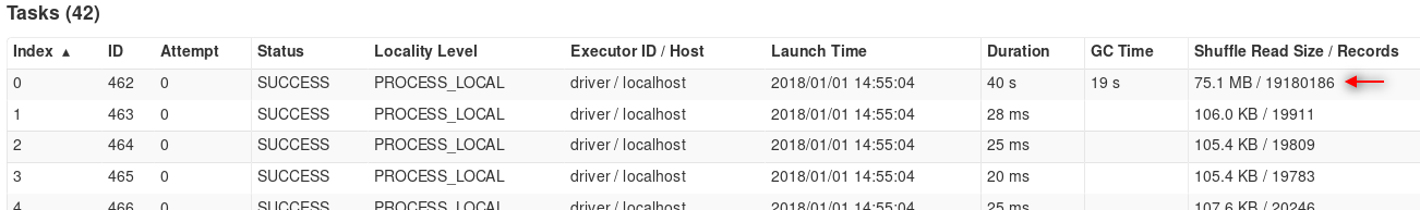
val input = sc.parallelize(1 to 1000, 42).keyBy(Math.min(_, 10))
val joined = input.cogroup(input)
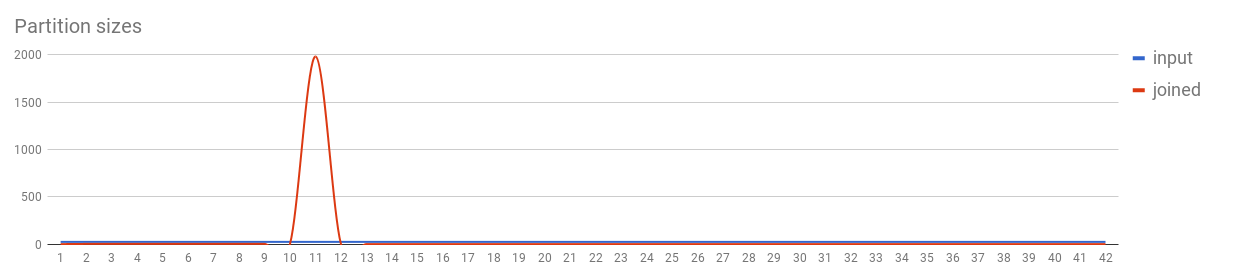
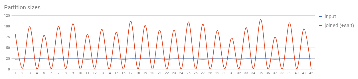
As the partitioning in these cases depends entirely on the selected key (specifically its Murmur3 hash), care has to be taken to avoid unusually large partitions being created for common keys (e.g. null keys are a common special case). An efficient solution is to separate the relevant records, introduce a salt (random value) to their keys and perform the subsequent action (e.g. reduce) for them in multiple stages to get the correct result.
val input1 = sc.parallelize(1 to 1000, 42).keyBy(Math.min(_, 10) + Random.nextInt(100) * 100)
val input2 = sc.parallelize(1 to 1000, 42).keyBy(Math.min(_, 10) + Random.nextInt(100) * 100)
val joined = input1.cogroup(input2)
Sometimes there are even better solutions, like using map-side joins if one of the datasets is small enough.
val input = sc.parallelize(1 to 1000000, 42)
val lookup = Map(0 -> "a", 1 -> "b", 2 -> "c")
val joined = input.map(x => x -> lookup(x % 3))
DataFrames and Datasets
The high-level APIs share a special approach to partitioning data. All data blocks of the input files are added into common pools, just as in wholeTextFiles, but the pools are then divided into partitions according to two settings: spark.sql.files.maxPartitionBytes, which specifies a maximum partition size (128MB by default), and spark.sql.files.openCostInBytes, which specifies an estimated cost of opening a new file in bytes that could have been read (4MB by default). The framework will figure out the optimal partitioning of input data automatically based on this information.
When it comes to partitioning on shuffles, the high-level APIs are, sadly, quite lacking (at least as of Spark 2.2). The number of partitions can only be specified statically on a job level by specifying the spark.sql.shuffle.partitions setting (200 by default).
The high-level APIs can automatically convert join operations into broadcast joins. This is controlled by spark.sql.autoBroadcastJoinThreshold, which specifies the maximum size of tables considered for broadcasting (10MB by default) and spark.sql.broadcastTimeout, which controls how long executors will wait for broadcasted tables (5 minutes by default).
Repartitioning
All of the APIs also provide two methods to manipulate the number of partitions. The first one is repartition which forces a shuffle in order to redistribute the data among the specified number of partitions (by the aforementioned Murmur hash). As shuffling data is a costly operation, repartitioning should be avoided if possible. There are also more specific variants of this operation: sortable pair RDDs have repartitionAndSortWithinPartitions which can be used with a custom partitioner, whereas DataFrames and Datasets have repartition with column parameters to control the partitioning characteristics.
The second method provided by all APIs is coalesce which is much more performant than repartition because it does not shuffle data but only instructs Spark to read several existing partitions as one. This, however, can only be used to decrease the number of partitions and cannot be used to change partitioning characteristics. There is usually no reason to use it, as Spark is designed to take advantage of larger numbers of small partitions, other than reducing the number of files on output or the number of batches when used together with foreachPartition (e.g. to send results to a database).
3. Serialization
Another thing that is tricky to take care of correctly is serialization, which comes in two varieties: data serialization and closure serialization. Data serialization refers to the process of encoding the actual data that is being stored in an RDD whereas closure serialization refers to the same process but for the data that is being introduced to the computation externally (like a shared field or variable). It is important to distinguish these two as they work very differently in Spark.
Data serialization
Spark supports two different serializers for data serialization. The default one is Java serialization which, although it is very easy to use (by simply implementing the Serializable interface), is very inefficient. That is why it is advisable to switch to the second supported serializer, Kryo, for the majority of production uses. This is done by setting spark.serializer to org.apache.spark.serializer.KryoSerializer. Kryo is much more efficient and does not require the classes to implement Serializable (as they are serialized by Kryo’s FieldSerializer by default). However, in very rare cases, Kryo can fail to serialize some classes, which is the sole reason why it is still not Spark’s default. It is also a good idea to register all classes that are expected to be serialized (Kryo will then be able to use indices instead of full class names to identify data types, reducing the size of the serialized data thereby increasing performance even further).
case class Test(a: Int = Random.nextInt(1000000),
                b: Double = Random.nextDouble,
                c: String = Random.nextString(1000),
                d: Seq[Int] = (1 to 100).map(_ => Random.nextInt(1000000))) extends Serializable

val input = sc.parallelize(1 to 1000000, 42).map(_ => Test()).persist(DISK_ONLY)
input.count() // Force initialization
val shuffled = input.repartition(43).count()
| RDD | Average time | Min. time | Max. time |
|---|---|---|---|
| java | 65990.9ms | 64482ms | 68148ms |
| kryo | 30196.5ms | 28322ms | 33012ms |
Lineage (Java):
(42) MapPartitionsRDD[1] at map at <console>:25 [Disk Serialized 1x Replicated]
 |        CachedPartitions: 42; MemorySize: 0.0 B; ExternalBlockStoreSize: 0.0 B; DiskSize: 3.8 GB
 |   ParallelCollectionRDD[0] at parallelize at <console>:25 [Disk Serialized 1x Replicated]
Lineage (Kryo):
(42) MapPartitionsRDD[1] at map at <console>:25 [Disk Serialized 1x Replicated]
 |        CachedPartitions: 42; MemorySize: 0.0 B; ExternalBlockStoreSize: 0.0 B; DiskSize: 3.1 GB
 |   ParallelCollectionRDD[0] at parallelize at <console>:25 [Disk Serialized 1x Replicated]
DataFrames and Datasets
The high-level APIs are much more efficient when it comes to data serialization as they are aware of the actual data types they are working with. Thanks to this, they can generate optimized serialization code tailored specifically to these types and to the way Spark will be using them in the context of the whole computation. For some transformations it may also generate only partial serialization code (e.g. counts or array lookups). This code generation step is a component of Project Tungsten which is a big part of what makes the high-level APIs so performant.
It is worth noting that Spark benefits from knowing the properties of applied transformations during this process as it can propagate information on which columns are being used throughout the job graph (predicate pushdown). When using opaque functions in transformations (e.g. Datasets’ map or filter) this information is lost.
val input = sc.parallelize(1 to 1000000, 42).map(_ => Test()).toDS.persist(org.apache.spark.storage.StorageLevel.DISK_ONLY)
input.count() // Force initialization
val shuffled = input.repartition(43).count()
| DataFrame | Average time | Min. time | Max. time |
|---|---|---|---|
| tungsten | 1102.9ms | 912ms | 1776ms |
Lineage:
(42) MapPartitionsRDD[13] at rdd at <console>:30 []
 |   MapPartitionsRDD[12] at rdd at <console>:30 []
 |   MapPartitionsRDD[11] at rdd at <console>:30 []
 |   *SerializeFromObject [assertnotnull(input[0, $line16.$read$$iw$$iw$Test, true]).a AS a#5, assertnotnull(input[0, $line16.$read$$iw$$iw$Test, true]).b AS b#6, staticinvoke(class org.apache.spark.unsafe.types.UTF8String, StringType, fromString, assertnotnull(input[0, $line16.$read$$iw$$iw$Test, true]).c, true) AS c#7, newInstance(class org.apache.spark.sql.catalyst.util.GenericArrayData) AS d#8]
+- Scan ExternalRDDScan[obj#4]
 MapPartitionsRDD[4] at persist at <console>:27 []
 |       CachedPartitions: 42; MemorySize: 0.0 B; ExternalBlockStoreSize: 0.0 B; DiskSize: 3.2 GB
 |   MapPartitionsRDD[3] at persist at <console>:27 []
 |   MapPartitionsRDD[2] at persist at <console>:27 []
 |   MapPartitionsRDD[1] at map at <console>:27 []
 |   ParallelCollectionRDD[0] at parallelize at <console>:27 []
Closure serialization
In most Spark applications, there is not only the data itself that needs to be serialized. There are also external fields and variables that are used in the individual transformations. Let’s consider the following code snippet:
val factor = config.multiplicationFactor
rdd.map(_ * factor)
Here we use a value that is loaded from the application’s configuration as part of the computation itself. However, as everything that happens outside the transformation function itself happens on the driver, Spark has to transport the value to the relevant executors. Spark therefore computes what’s called a closure to the function in map comprising of all external values that it uses, serializes those values and sends them over the network. As closures can be quite complex, a decision was made to only support Java serialization there. Serialization of closures is therefore less efficient than serialization of the data itself, however as closures are only serialized for each executor on each transformation and not for each record, this usually does not cause performance issues. (There is, however, an unpleasant side-effect of needing these values to implement Serializable.)
Variables in closures are pretty simple to keep track of. Where there can be quite a bit deal of confusion is using fields. Let’s look at the following example:
class SomeClass(d: Int) extends Serializable {
  val c = 1
  val e = new SomeComplexClass

  def closure(rdd: RDD[Int], b: Int): RDD[Int] = {
    val a = 0
    rdd.map(_ + a + b + c + d)
  }
}
Here we can see that a is just a variable (just as factor before) and is therefore serialized as an Int. b is a method parameter (which behaves as a variable too), so that also gets serialized as an Int. However c is a class field and as such cannot be serialized separately. That means that in order to serialize it, Spark needs to serialize the whole instance of SomeClass with it (so it has to extend Serializable, otherwise we would get a run-time exception). The same is true for d as constructor parameters are converted into fields internally. Therefore, in both cases Spark would also have to send the values of c, d and e to the executors. As e might be quite costly to serialize, this is definitely not a good solution. We can solve this by avoiding class fields in closures:
class SomeClass(d: Int) {
  val c = 1
  val e = new SomeComplexClass

  def closure(rdd: RDD[Int], b: Int): RDD[Int] = {
    val a = 0
    val sum = a + b + c + d
    rdd.map(_ + sum)
  }
}
Here we prepare the value by storing it in a local variable sum. This then gets serialized as a simple Int and doesn’t drag the whole instance of SomeClass with it (so it does not have to extend Serializable anymore).
Spark also defines a special construct to improve performance in cases where we need to serialize the same value for multiple transformations. It is called a broadcast variable and is serialized and sent only once, before the computation, to all executors. This is especially useful for large variables like lookup tables.
val broadcastMap = sc.broadcast(Map(0 -> "a", 1 -> "b", 2 -> "c"))
val input = sc.parallelize(1 to 1000000, 42)
val joined = input.map(x => x -> broadcastMap.value(x % 3))
Spark provides a useful tool to determine the actual size of objects in memory called SizeEstimator which can help us to decide whether a particular object is a good candidate for a broadcast variable.
4. Memory management
It is important for the application to use its memory space in an efficient manner. As each application’s memory requirements are different, Spark divides the memory of an application’s driver and executors into multiple parts that are governed by appropriate rules and leaves their size specification to the user via application settings.
Driver memory

Driver’s memory structure is quite straightforward. It merely uses all its configured memory (governed by the spark.driver.memory setting, 1GB by default) as its shared heap space. In a cluster deployment setting there is also an overhead added to prevent YARN from killing the driver container prematurely for using too much resources.
Executor memory

Executors need to use their memory for a few main purposes: intermediate data for the current transformation (execution memory), persistent data for caching (storage memory) and custom data structures used in transformations (user memory). As Spark can compute the actual size of each stored record, it is able to monitor the execution and storage parts and react accordingly. Execution memory is usually very volatile in size and needed in an immediate manner, whereas storage memory is longer-lived, stable, can usually be evicted to disk and applications usually need it just for certain parts of the whole computation (and sometimes not at all). For that reason Spark defines a shared space for both, giving priority to execution memory. All of this is controlled by several settings: spark.executor.memory (1GB by default) defines the total size of heap space available, spark.memory.fraction setting (0.6 by default) defines a fraction of heap (minus a 300MB buffer) for the memory shared by execution and storage and spark.memory.storageFraction (0.5 by default) defines the fraction of storage memory that is unevictable by execution. It is useful to define these in a manner most suitable for your application. If, for example, the application heavily uses cached data and does not use aggregations too much, you can increase the fraction of storage memory to accommodate storing all cached data in RAM, speeding up reads of the data. On the other hand, if the application uses costly aggregations and does not heavily rely on caching, increasing execution memory can help by evicting unneeded cached data to improve the computation itself. Furthermore, keep in mind that your custom objects have to fit into the user memory.
Spark can also use off-heap memory for storage and part of execution, which is controlled by the settings spark.memory.offHeap.enabled (false by default) and spark.memory.offHeap.size (0 by default) and OFF_HEAP persistence level. This can mitigate garbage collection pauses.
DataFrames and Datasets
The high-level APIs use their own way of managing memory as part of Project Tungsten. As the data types are known to the framework and their lifecycle is very well defined, garbage collection can be avoided altogether by pre-allocating chunks of memory and micromanaging these chunks explicitly. This results in great reuse of allocated memory, effectively eliminating the need for garbage collection in execution memory. This optimization actually works so well that enabling off-heap memory has very little additional benefit (although there is still some).
5. Cluster resources
The last important point that is often a source of lowered performance is inadequate allocation of cluster resources. This takes many forms from inefficient use of data locality, through dealing with straggling executors, to preventing hogging cluster resources when they are not needed.
Data locality
In order to achieve good performance, our application’s computation should operate as close to the actual data as possible, to avoid unneeded transfers. That means it is a very good idea to run our executors on the machines that also store the data itself. When using HDFS Spark can optimize the allocation of executors in such a way as to maximize this probability. We can, however, increase this even further by good design.
We can reduce the amount of inter-node communication required by increasing the resources of a single executor while decreasing the overall number of executors, essentially forcing tasks to be processed by a limited number of nodes. Take the following example resource distribution:
| num_executors | executor_cores | executor_memory |
|---|---|---|
| 15 | 1 | 1g |
| 5 | 3 | 3g |
| 3 | 5 | 5g |
In all of the instances, we’ll be using the same amount of resources (15 cores and 15GB of memory). However, as we reduce the overall number of executors, we also reduce the need to transport data between them. Making the third option usually the fastest. On the other hand, there can be limitations in I/O throughput on a node level, depending on the operations requested, so we cannot increase this indefinitely. For example, for HDFS I/O the number of cores per executor is thought to peak in performance at about five.
We can also tweak Spark’s configuration relating to locality when reading data from the cluster using the spark.locality.wait setting (3 seconds by default) and its subsections (same as spark.locality.wait by default). These define timeouts for locality-based scheduling (lowering locality restrictions when they are reached).
Dynamic allocation
Explicit application-wide allocation of executors can have its downsides. There are some instances in which we may not want to have a uniform number of executors for the duration of the whole computation but would instead want some scaling. There can be not enough resources available on the cluster at a given time but we would like to run our computation regardless, we may be processing a transformation that requires much less resources and would not like to hog more than we need, etc. This is where dynamic allocation comes in.
With dynamic allocation (enabled by setting spark.dynamicAllocation.enabled to true) Spark begins each stage by trying to allocate as much executors as possible (up to the maximum parallelism of the given stage or spark.dynamicAllocation.maxExecutors, infinity by default), where first stage must get at least spark.dynamicAllocation.initialExecutors (same as spark.dynamicAllocation.minExecutors or spark.executor.instances by default).
During computation, if an executor is idle for more than spark.dynamicAllocation.executorIdleTimeout (60 seconds by default) it gets removed (unless it would bring the number of executors below spark.dynamicAllocation.minExecutors (0 by default). This ensures that our application doesn’t needlessly occupy cluster resources when performing cheaper transformations.
In order to be able to enable dynamic allocation, we must also enable Spark’s external shuffle service. This acts as a separate server running on each machine in the cluster that is able to manage shuffle files when the appropriate executor is no longer around (has been removed or lost). This is also beneficial in case of losing executors (e.g. due to pre-emptions) as the shuffle data in question does not have to be recomputed.
Speculative execution
Sometimes, even though we do everything correctly, we may still get poor performance on a specific machine due to circumstances outside our control (heavy load not related to Spark, hardware failures, etc.). For these cases, we may instruct Spark to re-execute tasks automatically after it detects such stragglers. To do this, enable the spark.speculation setting. The detection routine can be configured using this set of settings: spark.speculation.interval defines how often to check for stragglers (100ms by default), spark.speculation.multiplier defines how many times slower do the stragglers have to be (1.5 by default) and spark.speculation.quantile defines the fraction of tasks that have to be completed until the detection routine kicks in (0.75 by default).
Conclusion
As you can see, designing a Spark application for performance can be quite challenging and every step of the way seems to take its toll in terms of increased complexity, reduced versatility or prolonged analysis of the specific use case. Fortunately, it is seldom required to implement all of them as typical Spark applications are not as performance-sensitive anyway. Furthermore, a great deal can be achieved just by using the high-level APIs (DataFrames or Datasets). Although the decision to use them has to be made very early in the development process as switching them is not trivial.
Additionally, there are many other techniques that may help improve performance of your Spark jobs even further. Namely GC tuning, proper hardware provisioning and tweaking Spark’s numerous configuration options.